Thread: [PERFORM] Fwd: Slow query from ~7M rows, joined to two tables of ~100 rows each
[PERFORM] Fwd: Slow query from ~7M rows, joined to two tables of ~100 rows each
From
Chris Wilson
Date:
Dear pgsql-performance list,

I think I've found a case where the query planner chooses quite a suboptimal plan for joining three tables. The main "fact" table (metric_value) links to two others with far fewer rows (like an OLAP/star design). We retrieve and summarise a large fraction of rows from the main table, and sort according to an index on that table, and I'd like to speed it up, since we will need to run this query many times per day. I would really appreciate your advice, thank you in advance!
The following SQL creates test data which can be used to reproduce the problem:
drop table if exists metric_pos;create table metric_pos (id serial primary key, pos integer);insert into metric_pos (pos) SELECT (random() * 1000)::integer from generate_series(1,100);create index idx_metric_pos_id_pos on metric_pos (id, pos);drop table if exists asset_pos;create table asset_pos (id serial primary key, pos integer);insert into asset_pos (pos) SELECT (random() * 1000)::integer from generate_series(1,100);drop TABLE if exists metric_value;CREATE TABLE metric_value(id_asset integer NOT NULL,id_metric integer NOT NULL,value double precision NOT NULL,date date NOT NULL,timerange_transaction tstzrange NOT NULL,id bigserial NOT NULL,CONSTRAINT cons_metric_value_pk PRIMARY KEY (id))WITH (OIDS=FALSE);insert into metric_value (id_asset, id_metric, date, value, timerange_transaction)select asset_pos.id, metric_pos.id, generate_series('2015-06-01'::date, '2017-06-01'::date, '1 day'), random() * 1000, tstzrange(current_timestamp, NULL) from metric_pos, asset_pos;CREATE INDEX idx_metric_value_id_metric_id_asset_date ON metric_value (id_metric, id_asset, date, timerange_transaction, value);
This is an example of the kind of query we would like to speed up:
SELECT metric_pos.pos AS pos_metric, asset_pos.pos AS pos_asset, date, valueFROM metric_valueINNER JOIN asset_pos ON asset_pos.id = metric_value.id_assetINNER JOIN metric_pos ON metric_pos.id = metric_value.id_metricWHEREdate >= '2016-01-01' and date < '2016-06-01'AND timerange_transaction @> current_timestampORDER BY metric_value.id_metric, metric_value.id_asset, date
This takes ~12 seconds from psql. Wrapping it in "SELECT SUM(value) FROM (...) AS t" reduces that to ~8 seconds, so the rest is probably data transfer overhead which is unavoidable.
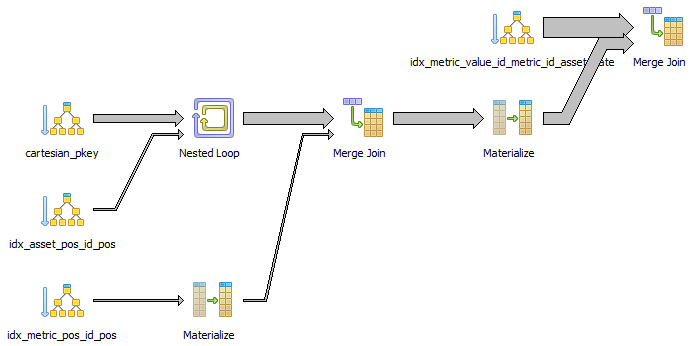
The actual query plan selected is (explain.depesz.com):
Sort (cost=378949.08..382749.26 rows=1520071 width=28) (actual time=7917.686..8400.254 rows=1520000 loops=1)Sort Key: metric_value.id_metric, metric_value.id_asset, metric_value.dateSort Method: external merge Disk: 62408kBBuffers: shared hit=24421 read=52392, temp read=7803 written=7803-> Hash Join (cost=3.31..222870.41 rows=1520071 width=28) (actual time=0.295..6049.550 rows=1520000 loops=1)Hash Cond: (metric_value.id_asset = asset_pos.id)Buffers: shared hit=24421 read=52392-> Nested Loop (cost=0.56..201966.69 rows=1520071 width=24) (actual time=0.174..4671.452 rows=1520000 loops=1)Buffers: shared hit=24420 read=52392-> Seq Scan on metric_pos (cost=0.00..1.50 rows=100 width=8) (actual time=0.015..0.125 rows=100 loops=1)Buffers: shared hit=1-> Index Only Scan using idx_metric_value_id_metric_id_asset_date on metric_value (cost=0.56..1867.64 rows=15201 width=20) (actual time=0.090..40.978 rows=15200 loops=100) Index Cond: ((id_metric = metric_pos.id) AND (date >= '2016-01-01'::date) AND (date < '2016-06-01'::date))Filter: (timerange_transaction @> now())Heap Fetches: 1520000Buffers: shared hit=24419 read=52392-> Hash (cost=1.50..1.50 rows=100 width=8) (actual time=0.102..0.102 rows=100 loops=1)Buckets: 1024 Batches: 1 Memory Usage: 12kBBuffers: shared hit=1-> Seq Scan on asset_pos (cost=0.00..1.50 rows=100 width=8) (actual time=0.012..0.052 rows=100 loops=1)Buffers: shared hit=1Planning time: 1.498 msExecution time: 8992.846 ms
Or visually:
What I find interesting about this query plan is:
The records can already be read in order from idx_metric_value.... If this was selected as the primary table, and metric_pos was joined to it, then the output would also be in order, and no sort would be needed.
We should be able to use a merge join to metric_pos, because it can be read in order of id_metric (its primary key, and the first column in idx_metric_value...). If not, a hash join should be faster than a nested loop, if we only have to hash ~100 records.
I think that the joins should be fairly trivial: easily held in memory and indexed by relatively small integers. They would probably be temporary tables in our real use case. But removing them (and just selecting the IDs from metric_value) cuts 4 seconds off the query time (to 3.3 seconds). Why are they slow?
If I remove one of the joins (asset_pos) then I get a merge join between two indexes, as expected, but it has a materialize just before it which makes no sense to me. Why do we need to materialize here? And why materialise 100 rows into 1.5 million rows? (explain.depesz.com)
SELECT metric_pos.pos AS pos_metric, id_asset AS pos_asset, date, valueFROM metric_valueINNER JOIN metric_pos ON metric_pos.id = metric_value.id_metricWHEREdate >= '2016-01-01' and date < '2016-06-01'AND timerange_transaction @> current_timestampORDER BY metric_value.id_metric, metric_value.id_asset, dateMerge Join (cost=0.70..209302.76 rows=1520071 width=28) (actual time=0.097..4899.972 rows=1520000 loops=1)Merge Cond: (metric_value.id_metric = metric_pos.id)Buffers: shared hit=76403-> Index Only Scan using idx_metric_value_id_metric_id_asset_date on metric_value (cost=0.56..182696.87 rows=1520071 width=20) (actual time=0.074..3259.870 rows=1520000 lo ops=1)Index Cond: ((date >= '2016-01-01'::date) AND (date < '2016-06-01'::date))Filter: (timerange_transaction @> now())Heap Fetches: 1520000Buffers: shared hit=76401-> Materialize (cost=0.14..4.89 rows=100 width=8) (actual time=0.018..228.265 rows=1504801 loops=1)Buffers: shared hit=2-> Index Only Scan using idx_metric_pos_id_pos on metric_pos (cost=0.14..4.64 rows=100 width=8) (actual time=0.013..0.133 rows=100 loops=1)Heap Fetches: 100Buffers: shared hit=2Planning time: 0.761 msExecution time: 5253.260 ms
The size of the result set is approximately 91 MB (measured with psql -c | wc -c). Why does it take 4 seconds to transfer this much data over a UNIX socket on the same box? Can it be made faster? The data is quite redundant (it's sorted for a start) so compression makes a big difference, and simple prefix elimination could probably reduce the volume of redundant data sent back to the client.
Standard background info:
- PostgreSQL 9.6.2 on x86_64-pc-linux-gnu, compiled by gcc (GCC) 4.8.5 20150623 (Red Hat 4.8.5-4), 64-bit, compiled from source.
- shared_buffers = 15GB, work_mem = 100MB, seq_page_cost = 0.5, random_page_cost = 1.0, cpu_tuple_cost = 0.01.
- HP ProLiant DL580 G7, Xeon(R) CPU E7- 4850 @ 2.00GHz * 80 cores, hardware RAID, 3.6 TB SAS array.
Thanks again in advance for any suggestions, hints or questions.
Cheers, Chris.
Attachment
[PERFORM] Re: Fwd: Slow query from ~7M rows, joined to two tables of ~100 rowseach
From
Karl Czajkowski
Date:
On Jun 23, Chris Wilson modulated:
> ...
>     create table metric_pos (id serial primary key, pos integer);
>     create index idx_metric_pos_id_pos on metric_pos (id, pos);
> ...
>     create table asset_pos (id serial primary key, pos integer);
> ...

Did you only omit a CREATE INDEX statement on asset_pos (id, pos) from
your problem statement or also from your actual tests?  Without any
index, you are forcing the query planner to do that join the hard way.


>     CREATE TABLE metric_value
>     (
>       id_asset integer NOT NULL,
>       id_metric integer NOT NULL,
>       value double precision NOT NULL,
>       date date NOT NULL,
>       timerange_transaction tstzrange NOT NULL,
>       id bigserial NOT NULL,
>       CONSTRAINT cons_metric_value_pk PRIMARY KEY (id)
>     )
>     WITH (
>       OIDS=FALSE
>     );
>
> ...
>     CREATE INDEX idx_metric_value_id_metric_id_asset_date ON
>     metric_value (id_metric, id_asset, date, timerange_transaction,
>     value);
> ...

Have you tried adding a foreign key constraint on the id_asset and
id_metric columns?  I wonder if you'd get a better query plan if the
DB knew that the inner join would not change the number of result
rows.  I think it's doing the join inside the filter step because
it assumes that the inner join may drop rows.

Also, did you include an ANALYZE step between your table creation
statements and your query benchmarks?  Since you are dropping and
recreating test data, you have no stats on anything.


> This is an example of the kind of query we would like to speed up:
>
>
>     SELECT metric_pos.pos AS pos_metric, asset_pos.pos AS pos_asset,
>     date, value
>     FROM metric_value
>     INNER JOIN asset_pos ON asset_pos.id = metric_value.id_asset
>     INNER JOIN metric_pos ON metric_pos.id = metric_value.id_metric
>     WHERE
>     date >= '2016-01-01' and date < '2016-06-01'
>     AND timerange_transaction @> current_timestamp
>     ORDER BY metric_value.id_metric, metric_value.id_asset, date
>

How sparse is the typical result set selected by these date and
timerange predicates?  If it is sparse, I'd think you want your
compound index to start with those two columns.

Finally, your subject line said you were joining hundreds of rows to
millions.  In queries where we used a similarly small dimension table
in the WHERE clause, we saw massive speedup by pre-evaluating that
dimension query to produce an array of keys, the in-lining the actual
key constants in the where clause of a main fact table query that
no longer had the join in it.

In your case, the equivalent hack would be to compile the small
dimension tables into big CASE statements I suppose...


Karl
Re: [PERFORM] Fwd: Slow query from ~7M rows, joined to two tables of ~100 rows each
From
Chris Wilson
Date:
Hi Karl,
Thanks for the quick reply! Answers inline.
My starting point, having executed exactly the preparation query in my email, was that the sample EXPLAIN (ANALYZE, BUFFERS) SELECT query ran in 15.3 seconds (best of 5), and did two nested loops.
On 24 June 2017 at 03:01, Karl Czajkowski <karlcz@isi.edu> wrote:
Also, did you include an ANALYZE step between your table creation
statements and your query benchmarks? Since you are dropping and
recreating test data, you have no stats on anything.
I tried this suggestion first, as it's the hardest to undo, and could also be done automatically by a background ANALYZE while I wasn't looking. It did result in a switch to using hash joins (instead of nested loops), and to starting with the metric_value table (the fact table), which are both changes that I thought would help, and the EXPLAIN ... SELECT speeded up to 13.2 seconds (2 seconds faster; best of 5 again).
Did you only omit a CREATE INDEX statement on asset_pos (id, pos) from
your problem statement or also from your actual tests? Without any
index, you are forcing the query planner to do that join the hard way.
I omitted it from my previous tests and the preparation script because I didn't expect it to make much difference. There was already a primary key on ID, so this would only enable an index scan to be changed into an index-only scan, but the query plan wasn't doing an index scan.
It didn't appear to change the query plan or performance.
Have you tried adding a foreign key constraint on the id_asset and
id_metric columns? I wonder if you'd get a better query plan if the
DB knew that the inner join would not change the number of result
rows. I think it's doing the join inside the filter step because
it assumes that the inner join may drop rows.
This didn't appear to change the query plan or performance either.
> This is an example of the kind of query we would like to speed up:
>
>
> SELECT metric_pos.pos AS pos_metric, asset_pos.pos AS pos_asset,
> date, value
> FROM metric_value
> INNER JOIN asset_pos ON asset_pos.id = metric_value.id_asset
> INNER JOIN metric_pos ON metric_pos.id = metric_value.id_metric
> WHERE
> date >= '2016-01-01' and date < '2016-06-01'
> AND timerange_transaction @> current_timestamp
> ORDER BY metric_value.id_metric, metric_value.id_asset, date
>
How sparse is the typical result set selected by these date and
timerange predicates? If it is sparse, I'd think you want your
compound index to start with those two columns.
I'm not sure what "sparse" means? The date is a significant fraction (25%) of the total table contents in this test example, although we're flexible about date ranges (if it improves performance per day) since we'll end up processing a big chunk of the entire table anyway, batched by date. Almost no rows will be removed by the timerange_transaction filter (none in our test example). We expect to have rows in this table for most metric and asset combinations (in the test example we populate metric_value using the cartesian product of these tables to simulate this).
I created the index starting with date and it did make a big difference: down to 10.3 seconds using a bitmap index scan and bitmap heap scan (and then two hash joins as before).
I was also able to shave another 1.1 seconds off (down to 9.2 seconds) by materialising the cartesian product of id_asset and id_metric, and joining to metric_value, but I don't really understand why this helps. It's unfortunate that this requires materialisation (using a subquery isn't enough) and takes more time than it saves from the query (6 seconds) although it might be partially reusable in our case.
CREATE TABLE cartesian ASSELECT DISTINCT id_metric, id_asset FROM metric_value;SELECT metric_pos.pos AS pos_metric, asset_pos.pos AS pos_asset, date, valueFROM cartesianINNER JOIN metric_value ON metric_value.id_metric = cartesian.id_metric AND metric_value.id_asset = cartesian.id_assetINNER JOIN asset_pos ON asset_pos.id = metric_value.id_assetINNER JOIN metric_pos ON metric_pos.id = metric_value.id_metricWHEREdate >= '2016-01-01' and date < '2016-06-01'AND timerange_transaction @> current_timestampORDER BY metric_value.id_metric, metric_value.id_asset, date;
And I was able to shave another 3.7 seconds off (down to 5.6 seconds) by making the only two columns of the cartesian table into its primary key, although again I don't understand why:
alter table cartesian add primary key (id_metric, id_asset);
This uses merge joins instead, which supports the hypothesis that merge joins could be faster than hash joins if only we can persuade Postgres to use them. It also contains two materialize steps that I don't understand.
Finally, your subject line said you were joining hundreds of rows to
millions. In queries where we used a similarly small dimension table
in the WHERE clause, we saw massive speedup by pre-evaluating that
dimension query to produce an array of keys, the in-lining the actual
key constants in the where clause of a main fact table query that
no longer had the join in it.
In your case, the equivalent hack would be to compile the small
dimension tables into big CASE statements I suppose...
Nice idea! I tried this but unfortunately it made the query 16 seconds slower (up to 22 seconds) instead of faster. I'm not sure why, perhaps the CASE expression is just very slow to evaluate?
SELECTcase metric_value.id_metric when 1 then 565 when 2 then 422 when 3 then 798 when 4 then 161 when 5 then 853 when 6 then 994 when 7 then 869 when 8 then 909 when 9 then 226 when 10 then 32 when 11then 592 when 12 then 247 when 13 then 350 when 14 then 964 when 15 then 692 when 16 then 759 when 17 then 744 when 18 then 192 when 19 then 390 when 20 then 804 when 21 then 892 when 22 then 219 when 23 then 48 when 24 then 272 when 25 then 256 when 26 then 955 when 27 then 258 when 28 then 858 when 29 then 298 when 30 then 200 when 31 then 681 when 32 then 862when 33 then 621 when 34 then 478 when 35 then 23 when 36 then 474 when 37 then 472 when 38 then 892 when 39 then 383 when 40 then 699 when 41 then 924 when 42 then 976 when 43 then946 when 44 then 275 when 45 then 940 when 46 then 637 when 47 then 34 when 48 then 684 when 49 then 829 when 50 then 423 when 51 then 487 when 52 then 721 when 53 then 642 when 54then 535 when 55 then 992 when 56 then 898 when 57 then 490 when 58 then 251 when 59 then 756 when 60 then 788 when 61 then 451 when 62 then 437 when 63 then 650 when 64 then 72 when65 then 915 when 66 then 673 when 67 then 546 when 68 then 387 when 69 then 565 when 70 then 929 when 71 then 86 when 72 then 490 when 73 then 905 when 74 then 32 when 75 then 764 when 76 then 845 when 77 then 669 when 78 then 798 when 79 then 529 when 80 then 498 when 81 then 221 when 82 then 16 when 83 then 219 when 84 then 864 when 85 then 551 when 86 then 211 when 87 then 762 when 88 then 42 when 89 then 462 when 90 then 518 when 91 then 830 when 92 then 912 when 93 then 954 when 94 then 480 when 95 then 984 when 96 then 869 when 97 then 153 when 98 then 530 when 99 then 257 when 100 then 718 end AS pos_metric,case metric_value.id_asset when 1 then 460 when 2 then 342 when 3 then 208 when 4 then 365 when 5 then 374 when 6 then 972 when 7 then 210 when 8 then 43 when 9 then 770 when 10 then 738 when 11then 540 when 12 then 991 when 13 then 754 when 14 then 759 when 15 then 855 when 16 then 305 when 17 then 970 when 18 then 617 when 19 then 347 when 20 then 431 when 21 then 134 when 22 then 176 when 23 then 343 when 24 then 88 when 25 then 656 when 26 then 328 when 27 then 958 when 28 then 809 when 29 then 858 when 30 then 214 when 31 then 527 when 32 then 318when 33 then 557 when 34 then 735 when 35 then 683 when 36 then 930 when 37 then 707 when 38 then 892 when 39 then 973 when 40 then 477 when 41 then 631 when 42 then 513 when 43 then469 when 44 then 385 when 45 then 272 when 46 then 324 when 47 then 690 when 48 then 242 when 49 then 940 when 50 then 36 when 51 then 674 when 52 then 74 when 53 then 212 when 54 then 17 when 55 then 163 when 56 then 868 when 57 then 345 when 58 then 120 when 59 then 677 when 60 then 202 when 61 then 335 when 62 then 204 when 63 then 520 when 64 then 891 when65 then 938 when 66 then 203 when 67 then 822 when 68 then 645 when 69 then 95 when 70 then 795 when 71 then 123 when 72 then 726 when 73 then 308 when 74 then 591 when 75 then 110 when 76 then 581 when 77 then 915 when 78 then 800 when 79 then 823 when 80 then 855 when 81 then 836 when 82 then 496 when 83 then 929 when 84 then 48 when 85 then 513 when 86 then 92when 87 then 916 when 88 then 858 when 89 then 213 when 90 then 593 when 91 then 60 when 92 then 547 when 93 then 796 when 94 then 581 when 95 then 438 when 96 then 735 when 97 then783 when 98 then 260 when 99 then 380 when 100 then 878 end AS pos_asset,date, valueFROM metric_valueWHEREdate >= '2016-01-01' and date < '2016-06-01'AND timerange_transaction @> current_timestampORDER BY metric_value.id_metric, metric_value.id_asset, date;
Thanks again for the suggestions :) I'm still very happy for any ideas on how to get back the 2 seconds longer than it takes without any joins to the dimension tables (3.7 seconds), or explain why the cartesian join helps and/or how we can get the same speedup without materialising it.
SELECT id_metric, id_asset, date, valueFROM metric_valueWHEREdate >= '2016-01-01' and date < '2016-06-01'AND timerange_transaction @> current_timestampORDER BY date, metric_value.id_metric;
Cheers, Chris.
Attachment
[PERFORM] Re: Fwd: Slow query from ~7M rows, joined to two tables of ~100 rowseach
From
Karl Czajkowski
Date:
On Jun 26, Chris Wilson modulated:
> ...
>     In your case, the equivalent hack would be to compile the small
>     dimension tables into big CASE statements I suppose...
>
>
> Nice idea! I tried this but unfortunately it made the query 16 seconds
> slower (up to 22 seconds) instead of faster.

Other possible rewrites to try instead of joins:

  -- replace the case statement with a scalar subquery

  -- replace the case statement with a stored procedure wrapping that scalar subquery
     and declare the procedure as STABLE or even IMMUTABLE

These are shots in the dark, but seem easy enough to experiment with and might
behave differently if the query planner realizes it can cache results for
repeated use of the same ~100 input values.


Karl
[PERFORM] Re: Fwd: Slow query from ~7M rows, joined to two tables of ~100 rowseach
From
Karl Czajkowski
Date:
On Jun 26, Chris Wilson modulated:

> I created the index starting with date and it did make a big
> difference: down to 10.3 seconds using a bitmap index scan and bitmap
> heap scan (and then two hash joins as before).
>

By the way, what kind of machine are you using?  CPU, RAM, backing
storage?

I tried running your original test code and the query completed in
about 8 seconds, and adding the index changes and analyze statement
brought it down to around 2.3 seconds on my workstation with Postgres
9.5.7.  On an unrelated development VM with Postgres 9.6.3, the final
form took around 4 seconds.


Karl
Re: [PERFORM] Fwd: Slow query from ~7M rows, joined to two tables of~100 rows each
From
Jeff Janes
Date:
On Fri, Jun 23, 2017 at 1:09 PM, Chris Wilson <chris+postgresql@qwirx.com> wrote:
The records can already be read in order from idx_metric_value.... If this was selected as the primary table, and metric_pos was joined to it, then the output would also be in order, and no sort would be needed.We should be able to use a merge join to metric_pos, because it can be read in order of id_metric (its primary key, and the first column in idx_metric_value...). If not, a hash join should be faster than a nested loop, if we only have to hash ~100 records.
Hash joins do not preserve order. They could preserve the order of their "first" input, but only if the hash join is all run in one batch and doesn't spill to disk. But the hash join code is never prepared to make a guarantee that it won't spill to disk, and so never considers it to preserve order. It thinks it only needs to hash 100 rows, but it is never absolutely certain of that, until it actually executes.
If I set enable_sort to false, then I do get the merge join you want (but with asset_pos joined by nested loop index scan, not a hash join, for the reason just stated above) but that is slower than the plan with the sort in it, just like PostgreSQL thinks it will be.
If I vacuum your fact table, then it can switch to use index only scans. I then get a different plan, still using a sort, which runs in 1.6 seconds. Sorting is not the slow step you think it is.
Be warned that "explain (analyze)" can substantially slow down and distort this type of query, especially when sorting. You should run "explain (analyze, timing off)" first, and then only trust "explain (analyze)" if the overall execution times between them are similar.
If I remove one of the joins (asset_pos) then I get a merge join between two indexes, as expected, but it has a materialize just before it which makes no sense to me. Why do we need to materialize here? And why materialise 100 rows into 1.5 million rows? (explain.depesz.com)
-> Materialize (cost=0.14..4.89 rows=100 width=8) (actual time=0.018..228.265 rows=1504801 loops=1)Buffers: shared hit=2-> Index Only Scan using idx_metric_pos_id_pos on metric_pos (cost=0.14..4.64 rows=100 width=8) (actual time=0.013..0.133 rows=100 loops=1)Heap Fetches: 100Buffers: shared hit=2
It doesn't need to materialize, it does it simply because it thinks it will be faster (which it is, slightly). You can prevent it from doing so by set enable_materialize to off. The reason it is faster is that with the materialize, it can check all the visibility filters at once, rather than having to do it repeatedly. It is only materializing 100 rows, the 1504801 comes from the number of rows the projected out of the materialized table (one for each row in the other side of the join, in this case), rather than the number of rows contained within it.
And again, vacuum your tables. Heap fetches aren't cheap.
The size of the result set is approximately 91 MB (measured with psql -c | wc -c). Why does it take 4 seconds to transfer this much data over a UNIX socket on the same box?
It has to convert the data to a format used for the wire protocol (hardware independent, and able to support user defined and composite types), and then back again.
> work_mem = 100MB
Can you give it more than that? How many simultaneous connections do you expect?
Cheers,
Jeff